What are we trying to figure out when we talk about a force field?
- What are the force lines look like? Diverging or twisting? How can we measure them?
- What would happen if two fields connected together?
- How can we know the effect of a field if we already knew something about the source? How can we know something about a source if we already knew the effect of the field it excited?
- How about the energy or something else?
By solving the above questions no.1 we can get some fundamental equations of the field. Questions no.3 are the basic problems that we need some solutions and questions no.1 and no.2 are of help. As for question no.4, that’s something matters in practical applications.
We can do those with our mathematical tools. However, every physics issue has to be started with some experiments. How much is the force? That is question no.0.
Now that I cannot demonstrate all the laws and formulas myself, I am going to list some pioneer scientists’ discoveries of three kinds of basic static electromagnetic fields below, and two of them are parts of electrostatics. What I can fully understand is that, these formulas are of simplicity and elegance undoubtedly.
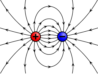
1. Static Electric field
The static electric field is produced by stationary charges, positive ones or negative ones.
a). Coulomb’s Law
First published by Charles Augustin de Coulomb in 1784.
$$\begin{aligned}
\vec{F_{1\to 2}}=\frac{q_{1}q_{2}}{4\pi \varepsilon_{0} |\vec{r_{2}}-\vec{r_{1}}|^2}\hat{e_{12}}=\frac{q_1 q_2(\vec{r_2}-\vec{r_1})}{4\pi \varepsilon_0 |\vec{r_2}-\vec{r_1}|^3}\\
\vec{F_{2\to 1}}=\frac{q_{1}q_{2}}{4\pi \varepsilon_{0} |\vec{r_{1}}-\vec{r_{2}}|^2}\hat{e_{21}}=\frac{q_1 q_2(\vec{r_1}-\vec{r_2})}{4\pi \varepsilon_0 |\vec{r_1}-\vec{r_2}|^3}
\end{aligned}$$
b). Electric Field Intensity ( $\vec{E}$ )
The electric field $\vec{E}$ at a given point is defined as the (vectorial) force $\vec{F}$ that would be exerted on a stationary test particle of unit charge by electromagnetic forces ( i.e. the Lorentz force ). A particle of charge q would be subject to a force: $$\vec{F}=q\cdot\vec{E}$$
c). Fundamental Equations
By using the mathematical tools we obtained last time ( flux, circulation, divergence, curl ), we are able to get some fundamental equations of static electric field: Gauss’s flux theorem and circuital theorem of static electric field, in both integral form and differential form.
$$\left\{
\begin{aligned}
&\oint_S \vec{E}\cdot d\vec{S}=\frac{Q}{\varepsilon_0}\\
&\oint_L \vec{E}\cdot d\vec{l}=0\\
\end{aligned}
\right.$$
$$\left\{
\begin{aligned}
&\nabla\cdot\vec{E}=\frac{\rho}{\varepsilon_0}\\
&\nabla\times\vec{E}=0\\
\end{aligned}
\right.$$
However, because of polarization, those above formulas can only be used in a vacuum, where has a simple permittivity: $\varepsilon_0$.
We have to take polarization density $\vec{P}$ into account. We define electric displacement $\vec{D}$ as:
$$\vec{D}=\varepsilon_0 \vec{E} + \vec{P}$$
( As for why it is called “displacement”, we will talk about it next time. )
If the medium is not only linear but also isotropic:
$$\vec{P}=\chi \varepsilon_0 \vec{E}$$
$$\vec{D}=(1+\chi)\varepsilon_0\vec{E}=\varepsilon_r\varepsilon_0 \vec{E}=\varepsilon \vec{E}$$
So here are the fundamental equations (final version):
$$\left\{
\begin{aligned}
&\oint_S \vec{D}\cdot d\vec{S}=\int_V \rho_f dV=Q_f\\
&\oint_L \vec{E}\cdot d\vec{l}=0\\
\end{aligned}
\right.$$
$$\left\{
\begin{aligned}
&\nabla\cdot\vec{D}=\rho_f\\
&\nabla\times\vec{E}=0\\
\end{aligned}
\right.$$
Now we have already known about the force and what the force lines look like: The static electric field is an irrotational field.
d). Electric Potential
Since the curl of a static electric field equals to zero, we can define a variable to measure the divergence of the field. Imagine a waterfall, we now know the velocity of the water, how can we get the height of each point in this “waterfall field”? BTW, we want the height of ground remain zero.
$$\vec{E}=-\nabla\varphi$$
e). Boundary Conditions
Near to the boundary line of two static electric fields:
$$\left\{
\begin{aligned}
&\vec{E}_{1t}=\vec{E}_{2t}\\
&\vec{D}_{2n}-\vec{D}_{1n}=\sigma_f\\
\end{aligned}
\right.$$
Represented with electric potential:
$$\left\{
\begin{aligned}
&\varphi_1=\varphi_2\\
&\varepsilon_2\frac{\partial\varphi_2}{\partial n}-\varepsilon_1\frac{\partial\varphi_1}{\partial n}=-\sigma_f\\
\end{aligned}
\right.$$
If both of the mediums are linear and isotropic, here we have the law of reflection:
$$\frac{tan\alpha_1}{tan\alpha_2}=\frac{\varepsilon_1}{\varepsilon_2}$$
f). Basic Questions
How can we know the effect of a field if we already knew something about the source? How can we know something about a source if we already knew the effect of the field it excited?
Answers:
- Coulomb’s law and $\vec{E}$.
- Coulomb’s law and $\vec{E}$ and integration ( for continuous objects ).
- Gauss’s flux theorem ( for symmetrical objects ).
- Boundary conditions, along with Poisson’s equation: $\nabla^2\varphi=-\frac{\rho_f}{\varepsilon}$, or Laplace’s equation: $\nabla^2\varphi=0$.
- Method of image charges ( for different mediums ).
g). Energy
Separated charges:
$$\begin{aligned}
&W=\frac{1}{2}\sum^{n}_{i=1} q_i \varphi_i\\
&\varphi_i=\sum^{n}_{j=1,j\neq i}\varphi_{ij}\\
\end{aligned}$$
Continuous charged body:
$$W=\frac{1}{2}\int_V \rho\varphi dV=\frac{1}{2}\int_V \vec{D}\cdot\vec{E}dV$$
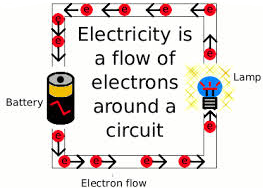
2. Steady Electric Field
We now know what would happen if we have some stationary charges. Next, we want to make them move, say, in a circuit. Although they are moving, the distribution of the charges is invariable. In that situation, we get a steady electric field.
a). Current Density
We can no longer regard currents as constants now. Current density is defined as a vector whose magnitude is the electric current per cross-sectional area at a given point in space.
$$\begin{aligned}
&\vec{J}=\rho \vec{\nu}\\
&I=\int_S \vec{J}\cdot d\vec{S}\\
\end{aligned}$$
b). Ohm’s Law: Differential Form
If the medium is linear and isotropic:
$$\begin{aligned}
\vec{J}=\gamma\vec{E}
\end{aligned}$$
$\gamma$ is the electrical conductivity of the medium.
c). KCL: Integral & Differential Form
We have already learned that the quantity of electric charges is conserved. Let’s consider a section of a electric wire. The current discharging from the section should equals to the decrement rate of charges.
$$\left\{
\begin{aligned}
&\oint_S \vec{J}\cdot d\vec{S}=-\int_V \frac{\partial\rho}{\partial t}dV\\
&\nabla \cdot \vec{J}=-\frac{\partial\rho}{\partial t}\\
\end{aligned}
\right.$$
The above equations are appropriate for any electric field. As for steady electric field, the equations become:
$$\left\{
\begin{aligned}
&\oint_S \vec{J}\cdot d\vec{S}=0\\
&\nabla \cdot \vec{J}=0\\
\end{aligned}
\right.$$
d). Fundamental Equations
Steady electric fields are not only irrotational, but also divergence-free.
Integral form:
$$\left\{
\begin{aligned}
&\oint_S \vec{J}\cdot d\vec{S}=0\\
&\oint_l \vec{E}\cdot d\vec{l}=0\\
\end{aligned}
\right.$$
Differential form:
$$\left\{
\begin{aligned}
\nabla \cdot \vec{J}=0\\
\nabla \times \vec{E}=0\\
\end{aligned}
\right.$$
e). Boundary Conditions
Near to the boundary line of two steady electric fields:
$$\left\{
\begin{aligned}
&\vec{E}_{1t}=\vec{E}_{2t}\\
&\vec{J}_{1n}=\vec{J}_{2n}\\
\end{aligned}
\right.$$
Represented with electric potential:
$$\left\{
\begin{aligned}
&\varphi_1=\varphi_2\\
&\gamma_1\frac{\partial\varphi_1}{\partial n}=\gamma_2\frac{\partial\varphi_2}{\partial n}\\
\end{aligned}
\right.$$
If both of the mediums are linear and isotropic, here we have the law of reflection:
$$\frac{tan\alpha_1}{tan\alpha_2}=\frac{\gamma_1}{\gamma_2}$$
That’s all… The calculations are quite exhausting. However, you can see the artistry.
References:
- Liu,Wenkai. Electromagnetic Fields and Electromagnetic Waves. [M]. Beijing: BUPT Press, 2013.
- Wikipedia [EB/OL]. https://en.wikipedia.org, 2016-03-05.