We have already learned something about electrostatics and magnetostatics. However these laws and formulas and equations are kind of complicated and messy. Real truths should not be something like those. They should be something like, you know, Newton’s Laws of motion. So, how can we simplify them? How can we unify them?

In a paper published in 1861: On physical lines of force, James Clerk Maxwell, a great Scottish scientist, gave us his answer. The equations in his papers were later improved and perfected, and named as Maxwell’s equations. Maxwell’s equations describe how electric and magnetic fields are generated and altered by each other and by charges and currents. These equations are a set of partial differential equations that, together with the Lorentz force law, form the foundation of classical electrodynamics, classical optics, and electric circuits.

Now let’s set these equations apart and give them some explanations.

1. Faraday’s Law of Induction

Electromagnetic induction was discovered by Michael Faraday in 1831. Michael Faraday explained electromagnetic induction using a concept he called lines of force. However, scientists at the time widely rejected his theoretical ideas, mainly because they were not formulated mathematically. An exception was Maxwell. In Maxwell’s papers, the time-varying aspect of electromagnetic induction is expressed as a differential equation which Oliver Heaviside ( him again :-D ) referred to as Faraday’s law even though it is different from the original version of Faraday’s law, and does not describe motional electromotive force.

As we already learned in high school, there are two kinds of electromotive forces, aka EMF.

One is generated by the movements of coils in constant magnetic fields ( motional EMF ), this is how a dynamo works:
$$\begin{aligned} \varepsilon=\oint_{l}(\vec{v}\times\vec{B})\cdot d\vec{l}=-\oint_{l}(\vec{B}\times\vec{v})\cdot d\vec{l} \end{aligned}$$
The other one is generated by the changing magnetic field, in which the coils are motionless ( induced EMF ), this is how a transformer works:
$$\begin{aligned} \varepsilon=-\frac{d\Psi}{dt}=-\frac{d}{dt}\int_{S}\vec{B}\cdot d\vec{S} \end{aligned}$$
There is a negative sign, because of Lenz’s law.

So, altogether:
$$\begin{aligned} \varepsilon=\oint_{l}(\vec{v}\times\vec{B})\cdot d\vec{l}-\frac{d}{dt}\int_{S}\vec{B}\cdot d\vec{S} \end{aligned}$$

We should note that electromotive forces are more essential than induced currents. Only in a conductor you can detect the induced currents, while you can get the electromotive forces on everything inside a magnetic field.

The above equations are born before Maxwell had his thoughts. What Maxwell did was: he assumed that there should be a surrounding electric field generated by every changing magnetic field. This kind of electric field, called induced electric field, can take some effect on electric charges.
$$\begin{aligned} \oint_l\vec{E_i}\cdot d\vec{l}=\oint_{l}(\vec{v}\times\vec{B})\cdot d\vec{l}-\frac{d}{dt}\int_{S}\vec{B}\cdot d\vec{S} \end{aligned}$$
The force lines of this kind of field are closed, not the same kind of force lines of a static electric field.

Then, Maxwell imagined the situation when a static electric field, generated by a static electric charge, and an induced electric field, excited by a changing magnetic field, coexist:
$$\begin{aligned} &\oint_l\vec{E}\cdot d\vec{l}=\oint_l\vec{E_i}\cdot d\vec{l}+\oint_l\vec{E_q}\cdot d\vec{l}\\ &\because\oint_l\vec{E_q}\cdot d\vec{l}=0\\ &\therefore\oint_l\vec{E}\cdot d\vec{l}=\oint_{l}(\vec{v}\times\vec{B})\cdot d\vec{l}-\frac{d}{dt}\int_{S}\vec{B}\cdot d\vec{S}\\ &\therefore\int_S\nabla\times\vec{E}\cdot d\vec{S}=-\int_S(\frac{\partial\vec{B}}{\partial t}-\nabla\times(\vec{v}\times\vec{B}))\cdot d{S}\\ &\therefore\nabla\times\vec{E}=\nabla\times(\vec{v}\times\vec{B})-\frac{\partial\vec{B}}{\partial t}\\ \end{aligned}$$
When the coils are not moving:
$$\begin{aligned} \nabla\times\vec{E}=-\frac{\partial\vec{B}}{\partial t} \end{aligned}$$
In integral form:
$$\begin{aligned} \oint_l\vec{E}\cdot d\vec{l}=-\int_S\frac{\partial\vec{B}}{\partial t}\cdot d\vec{S} \end{aligned}$$
These above two equations are the differential form and integral form of one of the four Maxwell’s equations: the Maxwell–Faraday equation.

2. Ampère’s Circuital Law

The previous equation tells us that magnetic fields can excite electric fields, now let’s consider whether electric fields can excite magnetic fields.

Actually we have learned the Ampère’s circuital law in magnetostatics:
$$\begin{aligned} \oint_{l}\vec{H}\cdot d\vec{l}=I \end{aligned}$$

However, this equation is false in some situations, like this: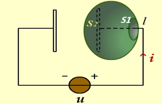

Here we have a plane-parallel capacitor in a circuit. If we use Ampère’s circuital law to calculate the current:
Through plane $S_{1}$:
$$\begin{aligned} \oint_{l}\vec{H}\cdot d\vec{l}=\int_{S_{1}}\vec{J}\cdot d\vec{S}=I \end{aligned}$$
Through plane $S_{2}$:
$$\begin{aligned} \oint_{l}\vec{H}\cdot d\vec{l}=\int_{S_{2}}\vec{J}\cdot d\vec{S}=0 \end{aligned}$$
Apparently, the currents should be equal. How can we resolve the contradiction?

Maxwell assumed that there is some kind of current passing through the capacitor, but this kind of current is not the common kind of current we can measure in a wire, it is displacement current. This kind of current is generated by a changing current, that’s why we are not aware of it if the current is steady in our circuit.

Of course, fields that generate displacement currents are called electric displacement field, the same $\vec{D}$ we used in magnetostatics.

These above two equations are the integral form and differential form of one of the four Maxwell’s equations: the Maxwell–Ampère equation.

3. Maxwell’s Equations

Now we know that electric fields and magnetic fields can activate each other and Maxwell used 2 of his 4 equations to explain this. The other 2 of his equations tell us the shapes of these fields, actually they are Guass’s Law and Gauss’s law for magnetism. We have learned those before.

So, as a whole, Maxwell’s equations are:
$$\left\{ \begin{aligned} &\nabla\cdot\vec{D}=\rho_{V}\\ &\nabla\cdot\vec{B}=0\\ &\nabla\times\vec{E}=-\frac{\partial\vec{B}}{\partial t}\\ &\nabla\times\vec{H}=\vec{J}+\frac{\partial\vec{D}}{\partial t}\\ \end{aligned} \right.$$
Or:
$$\left\{ \begin{aligned} &\oint_{S}\vec{D}\cdot d\vec{S}=Q\\ &\oint_{S}\vec{B}\cdot d\vec{S}=0\\ &\oint_{l}\vec{E}\cdot d\vec{l}=-\int_{S}\frac{\partial\vec{B}}{\partial t}\cdot d\vec{S}\\ &\oint_{l}\vec{H}\cdot d\vec{l}=\oint_{S}(\vec{J}+\frac{\partial\vec{D}}{\partial t})\cdot d\vec{S}=I\\ \end{aligned} \right.$$

By using these 4 equations, Maxwell simplified and unified electric fields and magnetic fields. They are all electromagnetic fields.

4. Boundary Conditions:

Just like what we’ve learned in electrostatic and magnetostatics:
$$\left\{ \begin{aligned} &\vec{E}_{1tan}=\vec{E}_{2tan}\\ &\vec{B}_{1nor}=\vec{B}_{2nor}\\ &\vec{D}_{2nor}-\vec{D}_{1nor}=\sigma_{f}\\ &\vec{H}_{1tan}-\vec{H}_{2tan}=\vec{K}\\ \end{aligned} \right.$$

5. The Speed of Light

Let’s do something else now. First, in a vacuum, the Maxwell’s equations become:
$$\left\{ \begin{aligned} &\nabla\times\vec{H}=\varepsilon\frac{\partial\vec{E}}{\partial t}\\ &\nabla\times\vec{E}=-\mu\frac{\partial\vec{H}}{\partial t}\\ &\nabla\cdot\vec{H}=0\\ &\nabla\cdot\vec{E}=0\\ \end{aligned} \right.$$

Let’s calculate the curls of each side of the first equation.
$$\begin{aligned} &\nabla\times\nabla\times\vec{H}=\nabla\times(\varepsilon\frac{\partial\vec{E}}{\partial t})\varepsilon\frac{\partial}{\partial t}(\nabla\times\vec{E}) \end{aligned}$$
Because of the identical equation we’ve learned in vector analysis:
$$\begin{aligned} \nabla\times\nabla\times\vec{H}=\nabla(\nabla\cdot\vec{H})-\nabla^{2}\vec{H} \end{aligned}$$
We can get the electromagnetic wave equation:
$$\begin{aligned} \nabla^{2}\vec{H}-\mu\varepsilon\frac{\partial^{2}\vec{H}}{\partial t^{2}}=0 \end{aligned}$$
For the same reason:
$$\begin{aligned} \nabla^{2}\vec{E}-\mu\varepsilon\frac{\partial^{2}\vec{E}}{\partial t^{2}}=0 \end{aligned}$$
Meanwhile, in our college physics class, we’ve learned the one-dimensional wave equation by analyzing the movement of a spring:
$$\begin{aligned} \frac{\partial^{2}y}{\partial x^{2}}-a^{2}\frac{\partial^{2}y}{\partial t^{2}}=0\\ (a=\frac{1}{v}) \end{aligned}$$
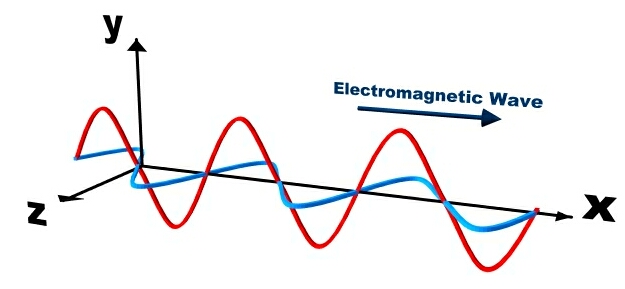
Therefore, we get the speed of electromagnetic wave in a vacuum:
$$\begin{aligned} v=\frac{1}{\sqrt{\mu_{0}\varepsilon_{0}}}\approx 3\times 10^{8} m/s \end{aligned}$$

Maxwell: Isn’t it just similar to the speed of light that Hippolyte Fizeau measured ?! How can this happen?! What is exactly inside a vacuum??

The results were:

First, Maxwell prophesied that light is electromagnetic radiation. This was later proved to be right by Heinrich Hertz in 1888.

Second, Maxwell’s thoughts facilitated the aether theories. This was later proved to be wrong by the Michelson–Morley experiment in 1880s.

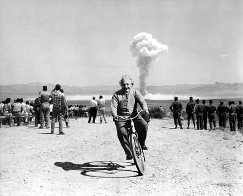
As for how Albert Einstein solved the problems left by aether theories by using his special relativity in 1905, that’s another long story.

References:

• Liu,Wenkai. Electromagnetic Fields and Electromagnetic Waves. [M]. Beijing: BUPT Press, 2013.
• He,Xiaoxiang. Engineering Electromagnetic Field. [M]. Beijing: Publishing House of Electronics Industry, 2011.
• Bhag Singh Guru. Electromagnetic Field Theory Fundamentals, 2nd ed. [M]. Cambridge: Cambridge University Press, 2009.
• Maxwell’s Equations [EB/OL]. http://www.maxwells-equations.com/, 2016-03-25.
• Guokr [EB/OL]. http://www.guokr.com/i/0867078073/, 2016-03-25.
• Wikipedia [EB/OL]. https://en.wikipedia.org, 2016-03-25.